Fitting a first-order or loglinear growth model using R
The data set “FirstOrder.csv” contains observations of microbial concentrations (log N) measured at different times (t) at a given environmental condition. Lets fit a first-order growth kinetics model \(log N = log N_0 + k \times t\) to the experimental data.
Let’s import the “FirstOrder.csv” dataset, and observe the first five lines.
dat <- read.csv("FirstOrder.csv", sep=";", header=TRUE)
dat
##    Time        N
## 1     0   37.298
## 2     1   56.149
## 3     2   81.580
## 4     3  108.758
## 5     4  147.276
## 6     5  197.160
## 7     6  273.014
## 8     7  368.254
## 9     8  490.822
## 10    9  673.304
## 11   10  909.398
## 12   11 1204.429
## 13   12 1640.532
## 14   13 2218.299
## 15   14 2983.926
## 16   15 4033.458
Plot N against Time, and observe that the relationship between the two variables is non-linear.
plot(dat$Time, dat$N, xlab="Time (hours)", ylab="N (cells/g)")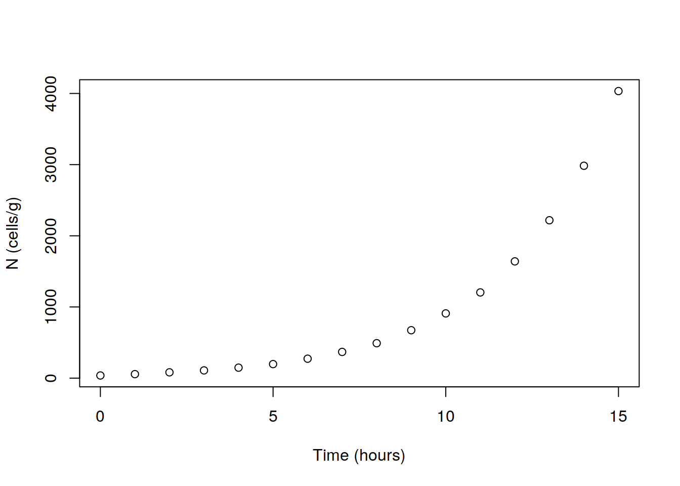
Take the logarithm of the variable N and add the new variable logN in the data set.
dat$logN <- log10(dat$N)
dat[1:5,]
##   Time       N     logN
## 1    0  37.298 1.571686
## 2    1  56.149 1.749342
## 3    2  81.580 1.911584
## 4    3 108.758 2.036461
## 5    4 147.276 2.168132
Now plot logN against Time, and observe that they have now a linear relationship.
plot(dat$Time, dat$logN, xlab="Time (hours)", ylab="log N (cels/g)")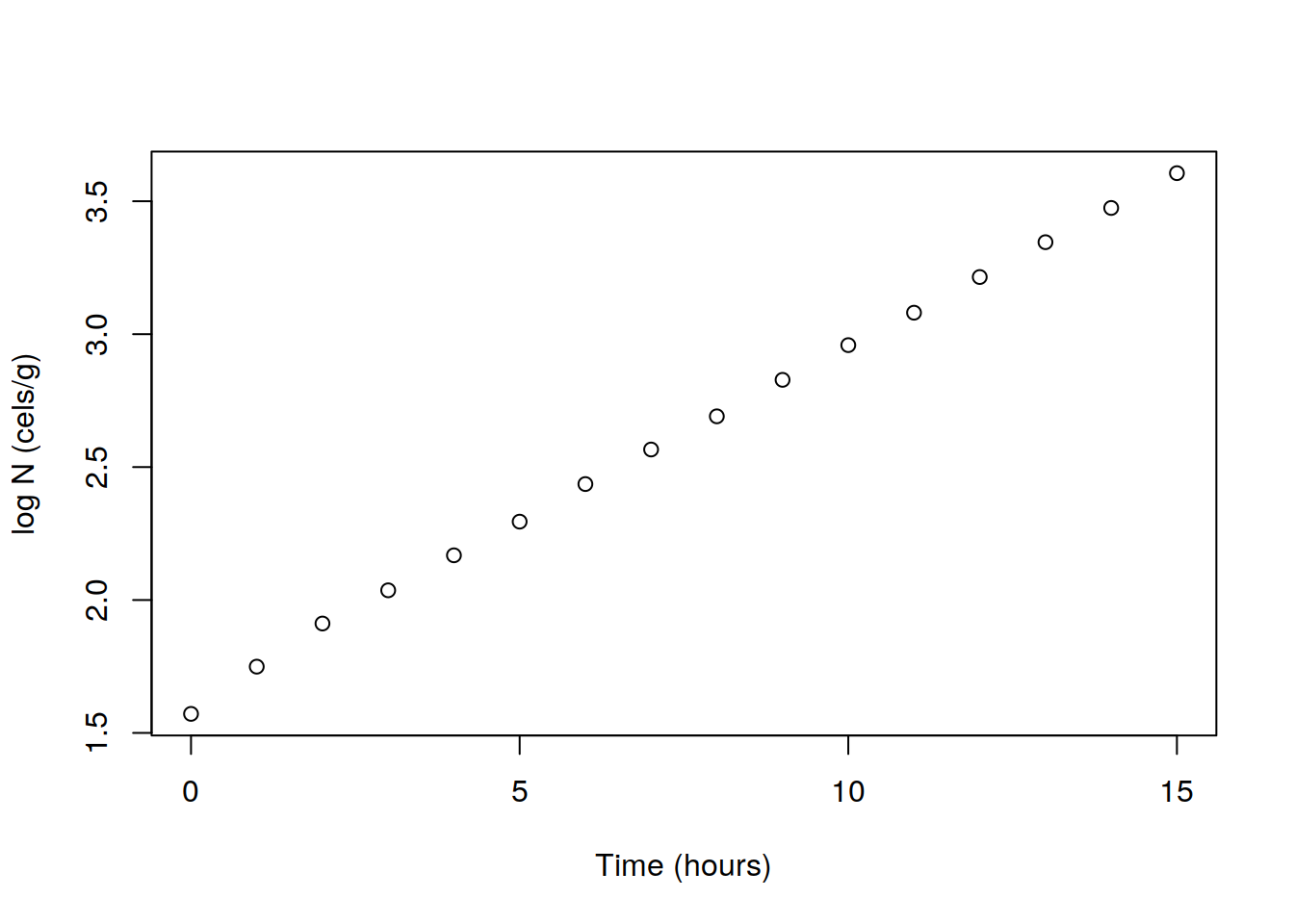
The first-order kinetics model is defined as Nt = N0*exp(k*t), then the log-linear model becomes ln(Nt) = ln(N0) + k*t. Fit a linear model using the lm() (linear models) function.
lm1 <- lm(logN ~ Time, data=dat)The results can be summarised using the summary() fucntion.
summary(lm1)
##
## Call:
## lm(formula = logN ~ Time, data = dat)
##
## Residuals:
##       Min        1Q    Median        3Q       Max
## -0.052876 -0.006170  0.004664  0.011795  0.021331
##
## Coefficients:
##              Estimate Std. Error t value Pr(>|t|)
## (Intercept) 1.6245612  0.0084968   191.2   <2e-16 ***
## Time        0.1328460  0.0009652   137.6   <2e-16 ***
## ---
## Signif. codes:  0 '***' 0.001 '**' 0.01 '*' 0.05 '.' 0.1 ' ' 1
##
## Residual standard error: 0.0178 on 14 degrees of freedom
## Multiple R-squared:  0.9993, Adjusted R-squared:  0.9992
## F-statistic: 1.894e+04 on 1 and 14 DF,  p-value: < 2.2e-16
You can add fitted values to the original data set.
dat$fitted <- fitted(lm1)
dat[1:5,]
##   Time       N     logN   fitted
## 1    0  37.298 1.571686 1.624561
## 2    1  56.149 1.749342 1.757407
## 3    2  81.580 1.911584 1.890253
## 4    3 108.758 2.036461 2.023099
## 5    4 147.276 2.168132 2.155945
Plot the observations against time and superimpose a fitted line. First, extract the model’s parameters and use the model to draw a fitted line.
coefs <- coef(lm1)
coefs
## (Intercept)        Time
##    1.624561    0.132846
logN0 <- coefs[1]
logN0
## (Intercept)
##    1.624561
k <- coefs[2]
k
##     Time
## 0.132846
Plot observed versus fitted values.
plot(dat$logN ~ dat$Time, data=dat,
     xlab="Time (hours)", ylab="log N (cells/g)")
time.levels <- seq(0, 20, by=1)
lines(time.levels, logN0 + k*time.levels, lty = 2, col = "blue")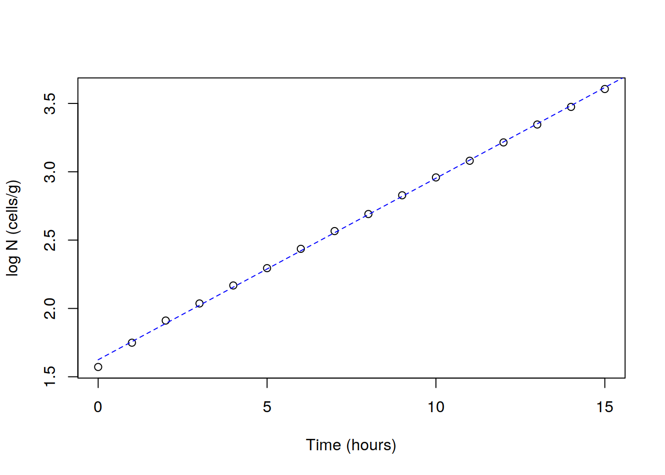
Vasco Cadavez
Professor of Animal Science
My research interests include: Animal Breeding, Food Safety Modelling, Statistical Modelling and Data Science.