Fitting a reparameterised Gompertz growth model using R
Using the data set “gomp1.csv”, find the parameters of the reparameterised Gompertz model.
\[\begin{equation} y= y_0 + (y_{max} -y_0)*exp(-exp(k*(lag-x)/(y_{max}-y_0) + 1) ) \end{equation}\]
Import the data set.
dat <- read.csv("gomp1.csv", sep=";", header=T)
plot(dat$Time, dat$logN)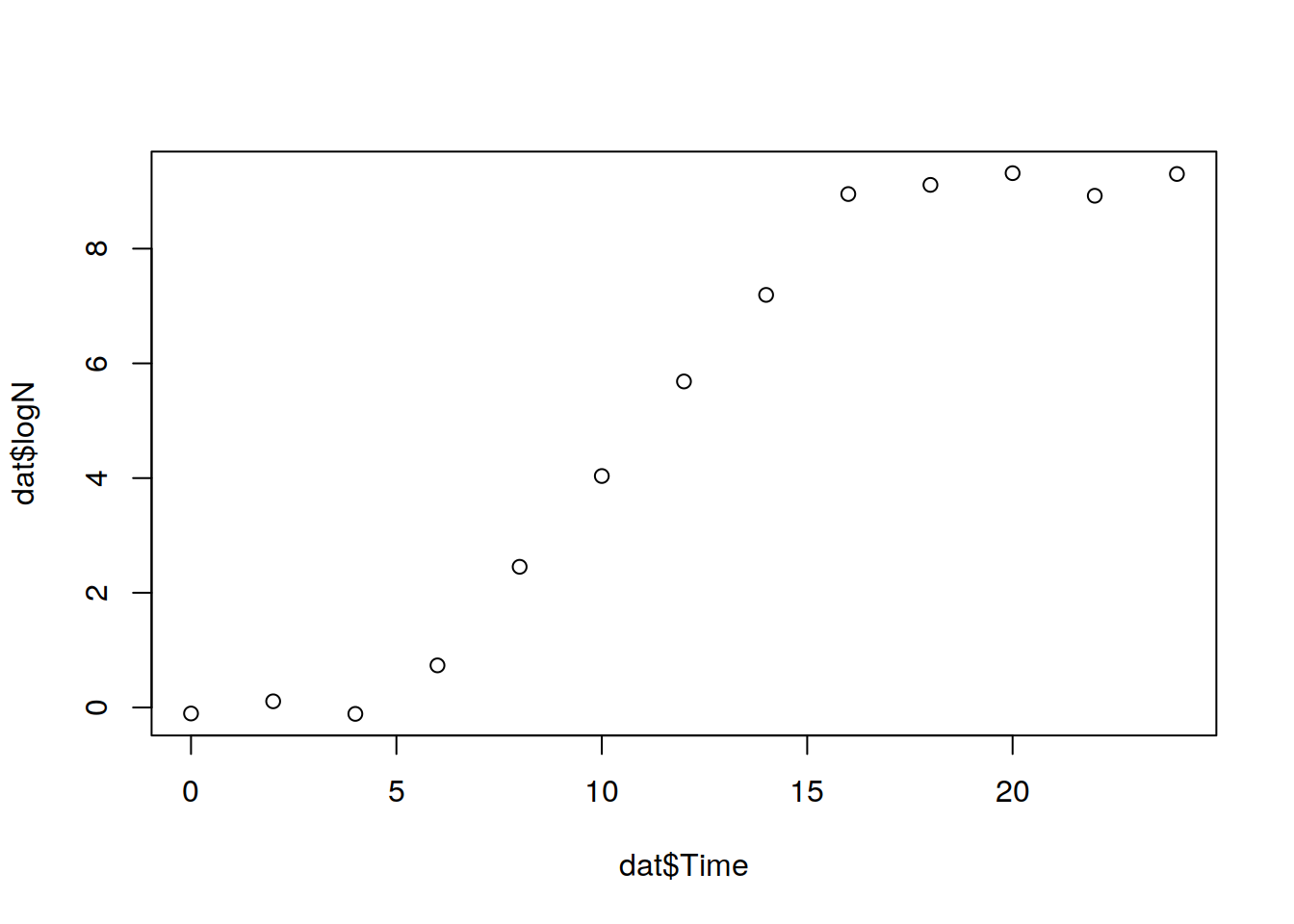
str(dat)
## 'data.frame':    13 obs. of  2 variables:
##  $ Time: int  0 2 4 6 8 10 12 14 16 18 ...
##  $ logN: num  -0.105 0.108 -0.111 0.734 2.453 ...
The next step is define the Gompertz function.
# Gompertz function
Gompertz <- function(x, y0, ymax, k, lag){
      result <- y0 + (ymax -y0)*exp(-exp(k*(lag-x)/(ymax-y0) + 1) )
      return(result)
      }
Check data by plot.
plot( logN ~ Time, data=dat, xlim=c(-1, 25), ylim=c(-1, 10))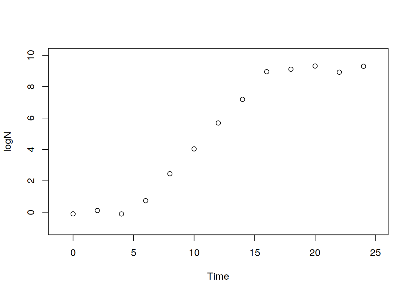
Fit the model to data using the nls() funtion and extract the models parameters.
Gomp1 <-  nls(logN ~ Gompertz(Time, y0, ymax, k, lag),
               data = dat,
               start = list(y0=0.15, ymax=7, k=0.5, lag=3))
# ectract model parameters
coefs <- coef(Gomp1)
coefs
##          y0        ymax           k         lag
## -0.02517334  9.60030027  2.78548012  5.88823263
y0   <- coefs[1]
y0
##          y0
## -0.02517334
ymax <- coefs[2]
ymax
##   ymax
## 9.6003
k   <- coefs[3]
k
##       k
## 2.78548
lag <- coefs[4]
lag
##      lag
## 5.888233
Now, plot the observed values against the fitted values.
time.levels <- seq(0, 24, by=0.1)
pred <- predict(Gomp1, list(x=time.levels) )
plot(logN ~ Time, data=dat, xlim=c(0,24), ylim=c(0, 10),
     main = "Fitted Gompertz model",
     sub = "Blue: fit; green: known")
lines(time.levels, Gompertz(time.levels,
                            y0 = y0, ymax = ymax, k = k, lag=lag),
      lty = 1, col = "red")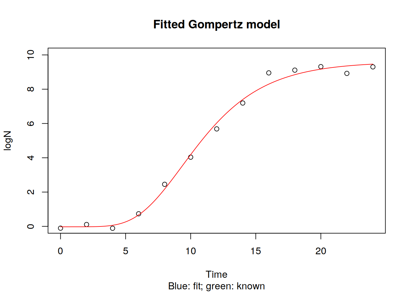
Add the confidence interval to the line offitted values.
library(nlme)
library(twNlme)
Gomp11 <- gnls(logN ~ y0 + (ymax -y0)*exp(-exp(k*(lag-Time)/(ymax-y0) + 1) ),
              data = dat,
              start = list(y0=-0.025, ymax=9.5, k=2.7, lag=5.8))
Gomp11
## Generalized nonlinear least squares fit
##   Model: logN ~ y0 + (ymax - y0) * exp(-exp(k * (lag - Time)/(ymax - y0) +      1))
##   Data: dat
##   Log-likelihood: -2.123991
##
## Coefficients:
##          y0        ymax           k         lag
## -0.02511771  9.60008391  2.78571200  5.88858202
##
## Degrees of freedom: 13 total; 9 residual
## Residual standard error: 0.3424286

# automatic derivation with accounting for residual variance model
nlmeFit <- attachVarPrep(Gomp11, fVarResidual=varResidPower)

newData <- data.frame( Time= seq(0,24,by=0.1))

resNlme <- varPredictNlmeGnls(Gomp11, newData)

# plotting prediction and standard errors
plot( logN ~ Time, dat, ylab="log CFU",
      xlim=c(0,24), ylim=c(-1, 10))
par(new=T)
plot( resNlme[,"fit"] ~ Time, newData, ylab="",
      type="l", xlim=c(0,24), ylim=c(-1, 10), lty="solid")
lines( resNlme[,"fit"]+resNlme[,"sdInd"] ~ Time, newData,
       col="orange", lty="dashed"  )
lines( resNlme[,"fit"]-resNlme[,"sdInd"] ~ Time, newData,
       col="orange", lty="dashed" )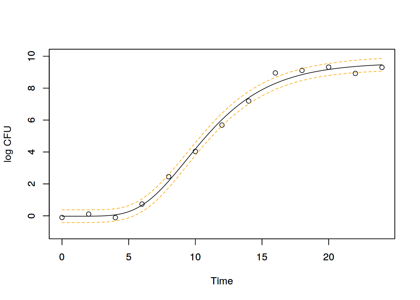
Vasco Cadavez
Professor of Animal Science
My research interests include: Animal Breeding, Food Safety Modelling, Statistical Modelling and Data Science.